NIPS - Day 6

This was the final day of the NIPS conference and the day of the workshop on Machine Learning for Sustainability; the workshop I submitted my paper to. It's a bit of a shame it came on the day when I think everyone was the most tired, but I think that's just a reality of post conference workshops. In general, the workshop mostly covered three main topics: climate modelling, energy and environmental management.

For me, the best part of this workshop was the chance to meet other researchers working on the problem of energy disaggregation. The workshop was organised by Zico Kolter, with an invited talk given by Mario Bergés, both of whom have published in this area and their papers have ended up on my reading list.

The morning invited talks were:

• Mario Bergés - Machine Learning Challenges in Building Energy Management: Energy Disaggregation as an Example
• Andreas Krause - Dynamic Resource Allocation in Conservation Planning

Before the midday break were the spotlights and poster session. These sessions were my first chance to present my work to the an external academic community and receive feedback, which was an absolutely invaluable opportunity. I tried my best to balance my time between presenting my poster to others and also to discuss the other posters with their authors. I was really impressed with the quality of the accepted papers, and hope this is indicative of the future of the MLSUST workshop.

The afternoon invited talks were:

• Drew Purves - Enabling Intelligent Management of the Biosphere
• Claire Monteleoni - Climate Informatics
• Kevin Swersky - Machine Learning for Hydrology, Water Monitoring and Environmental Sustainability
• Alex Rogers - Putting the “Smarts” into the Smart Grid: A Grand Challenge for Artificial Intelligence

The concluding session of the workshop was a panel discussion regarding the future of MLSUST. Much of the discussion was centered around the naming of the workhop, and whether sustainability represented the variety of topics in the workshop, but also whether the term encouraged researchers from other fields to submit and attend. Other ideas to promote interest in the workshop were raised, namely: well defined problems, competitions and data sets.

For me, the workshop was a brilliant venue to receive feedback on my PhD work, and for that I owe the organisers thanks.

NIPS - Day 5

I woke up on the first day of workshops to a beautiful sunrise in Sierra Nevada. I'm not sure what it is about mountain weather that causes the sky to turn so pink, but I'm definitely not complaining.

The NIPS organisers seem to have set it in stone that the each workshop will have a 5 hour break in the middle of the day for sleeping/skiing. As much as the 7.30am workshop starts hurt, I have to say I thoroughly enjoyed the opportunity to ski. I'm not sure that the schedule helped to sync the body clock with Spanish eating times, but I think a lot of people are jet lagged enough for that not to matter.

I attended the workshop on Decision Making with Multiple Imperfect Decision Makers. The two talks I enjoyed the most were:

• David Leslie - Random Belief Learning
• Stephen Roberts - Bayesian Combination of Multiple, Imperfect Classifiers

I also spoke to Edwin during the coffee breaks about how crowdsourcing is used to aggregate multiple data sources with of different quality, reliability etc. This prompted the thought that maybe something similar could be used in NIALM to collect large sets of appliance signatures. In my opinion, this would make a far more powerful data set for building generalisable appliance models than it would be for evaluating the performance of NIALM approaches.

NIPS - Day 4

Today was the final day of the main track, with only a morning of talks scheduled. Apart from some interesting but less relevant talks about the brain, I thought this one was pretty good:

• Continuous-Time Regression Models for Longitudinal Networks

After the morning sessions was the NIPS organised tour of the Alhambra. Moving over 1000 people around in coaches was always going to be a logistical nightmare, so it was no surprise loading/unloading took longer than planned. The tour of the Alhambra was excellent, and I've put a few photos at the bottom of this post to prove it. After the tour we set off up the mountains towards Sierra Nevada for two days of workshops. As the gradient increased our bus started to struggle, and when the road widened to two lanes the other buses stormed past us. However, the bus did its job, and we arrived in Sierra Nevada not too long after the others.

NIPS - Day 3

Today was another great day at NIPS, although I think the long days are starting to take their toll. The sessions were pretty cool, with some some great invited talks. I even noticed a few crowdsourcing papers making their way into NIPS, which I've already passed on to people in my group who might be interested.

Instead of the standard restaurant lunch, I decided to try to make the most of my last full day in Granada and go on a walk around the old town. There was so much stuff I would have missed I had not have strayed far from the conference venue, so really glad I made the effort. I took a few photos on my phone which I've stuck at the bottom of this post.

In the poster session I found one paper that was particularly relevant to what I do:

• Selective Prediction of Financial Trends with Hidden Markov Models

I think the method used for deciding whether to predict outcomes in financial markets is similar to the way in which our approach ignores observations from other appliances described in our paper. Their method of expanding single states of the Markov process to add more detail was also really interesting. I'll have to read their full paper when I get a little more time.

Tomorrow morning contains the last of the sessions at the main conference, followed by a visit to Granada's famous Alhambra. We then make the bus journey up the mountain to the workshops is Sierra Nevada.

NIPS - Day 2

Today was the first full day of NIPS, consisting of many spotlight and oral sessions. This has been my first experience of spotlight sessions, and I've been really impressed at how many new techniques I'm introduced to and how many thoughts about my own work it triggers. I have to say I much prefer it to the topic sessions I experienced at IJCAI.

I also learnt today that there's three identical (I think) Machine Learning Summer Schools (MLSS) held in different parts of the world. I attended the European Agent Systems Summer School (EASSS) 2011, and although it was really helpful in understanding other research in my group, it wasn't too relevant to my PhD. I think I'll look into MLSS to see whether it will be beneficial for me to attend it in 2012.

After attending the poster session I've also learnt the following:

• A0 is the best poster size (at least at NIPS). A1 posters are too small by comparison, while bigger posters require kneeling to read the bottom.
• People (or at least just myself) are most likely to view your poster if both of the following are true:
• a) something in your title interests them and
• b) your abstract confirms this. This might seem obvious, but it's interesting when you consider this along with acceptance likelihood and post publishing usefulness when writing your title and abstract.

Apart from this general conference waffle, I also came across the following interesting posters:

• Message parsing for approximate MAP inference with latent variables
• Comparative analysis of Viterbi training and maximum likelihood estimation for HMMs

NIPS - Day 1

After a long day of travelling yesterday, I arrived in Granada for NIPS2011. NIPS stands for Neural Information Processing Systems, and is widely regarded as the top machine learning conference. I'm here to present my paper, although that's not until the sustainability workshop on Saturday.

Today I attended 3 tutorials:

• Linear Programming Relaxations for Graphical Models
• Modern Bayesian Nonparametrics
• Graphical Models for the Internet

I really enjoyed each one, as the quality of presentation resulted in some really interesting and accessible tutorials.

I also went for lunch with a bunch of PhD students from the machine learning labs at Oxford, Cambridge and UCL, which was great to meet them and get a feel for what problems they're studying. We ate some interesting Paella, but I don't think it was quite good enough to warrant a return trip tomorrow.

After the welcome talk, there was a tapas reception and the first poster session. I spoke to many, many people who were using HMMs or similar graphical models in their work, which might even lead to some extensions to the paper I'm currently writing...

REDD Statistics

To allow the empirical comparison of different approaches to NIALM, a team at MIT built the Reference Energy Disaggregation Data set (REDD):
http://redd.csail.mit.edu/
Described in the paper:
Kolter JZ, Johnson MJ. REDD : A Public Data Set for Energy Disaggregation Research. In: Workshop on Data Mining Applications in Sustainability (SIGKDD). San Diego, CA; 2011

A few months ago I wrote a post giving some high level details about the data set, and since then, I've spent some time using it to benchmark various approaches. However, I've made many mistakes along the way, which were often due to lack of understanding of the data set. Due to the vastness of the data it's often hard to understand simple results, such as which appliances consume the most energy, or how long each house has been monitored. To tackle such confusion, I set about calculating a bunch of statistics and generating visualisations which I decided to share with the world through this post. For all the statistics below, I used the low frequency data (1 reading per second).

Houses

The data set contains 6 houses, for each of which I generated the following statistics:

House	Up Time (days)	Reliability (%)	Average Energy Consumption (kWh/day)
1	18	99.97	9.22
2	14	99.98	5.53
3	16	99.87	10.7
4	19	99.99	8.42
5	3	99.86	14.9
6	10	97.50	11.4

• Up time - duration for which mains power measurements are available at 1 second intervals
• Reliability - percentage of readings which are available at 1 second intervals
• Average energy consumption - the average energy consumed by each house's mains circuits

These statistics were calculated to give an overall view of the data collected for each house. However, I noticed that each house had data collected over different periods. Below is a plot of the up time of each house's mains circuit monitor:

Appliances

Each house contains between 11 and 26 circuit meters, each of which monitor one of the two phases of electricity input or one of the house's internal circuits. In my opinion, the importance of disaggregating an appliance varies according to its energy consumption, and therefore it's helpful to know how much energy each appliance type generally consumes when it is present in a house. This led me to generating the following statistics:

Appliance	Number of Houses Present In	Average Energy Consumption (kWh/day)	Percentage of Household Energy
Air conditioning	2	1.62	0.5
Bathroom GFI	5	0.15	5.4
Dishwasher	6	0.24	4.5
Disposal	3	0.00	8.6
Electric heater	3	0.62	1.3
Electronics	3	1.00	9.0
Furnace	3	1.32	8.6
Kitchen outlets	6	0.68	4.5
Lighting	6	2.02	4.5
Microwave	4	0.33	6.5
Miscellaneous	1	0.03	0.0
Outdoor outlets	1	0.00	2.7
Outlets unknown	4	0.37	6.7
Oven	1	0.27	0.0
Refrigerator	5	1.58	5.4
Smoke alarms	2	0.01	11.6
Stove	4	0.09	0.3
Subpanel	1	1.52	2.7
Washer/dryer	6	0.52	4.5

A problem with the average energy consumption and percentage of household energy consumption columns is that although an appliance might be present in a house, it might not be used. This has a major affect on the average given that we only have 6 houses.

Houses and Appliances

A more reliable source of information is to consider each house individually, and examine on average how much energy each appliance consumes.

                                       Average Energy Consumption (kWh/day)

Appliance	1	2	3	4	5	6
Air conditioning				0.004023		3.236165
Bathroom GFI	0.155818		0.406498	0.026811	0.083836	0.094664
Dishwasher	0.586979	0.214069	0.169982	0.186737	0.260919	0.005581
Disposal		0.001954	0.002056		0.001381
Electric heater	0.002869				1.342452	0.500762
Electronics			2.478051		0.410446	0.116638
Furnace			0.354939	2.368171	1.248476
Kitchen outlets	1.397504	0.394875	0.348328	1.639216	0.147725	0.181511
Lighting	1.850006	0.636832	2.222016	1.474698	3.235403	2.713484
Microwave	0.504392	0.367756	0.196976		0.241313
Miscellaneous				0.028333
Outdoor outlets					0.000882
Outlets unknown			0.160546	0.014136	0.295022	1.010813
Oven	0.266246
Refrigerator	1.360893	1.912154	1.126372		1.661399	1.845720
Smoke alarms			0.022473	0.000646
Stove	0.012405	0.034468		0.204273		0.103160
Subpanel					1.524733
Washer/dryer	0.972989	0.051357	1.876719	0.142617	0.006250	0.063892

I know this is mostly just raw statistics, so I'll look into some visualisations of this soon.

Paper accepted at NIPS2011 MLSUST workshop

I recently had a paper accepted at the 2011 Neural Information Processing Systems workshop on Machine Learning for Sustainability. The paper is titled Using Hidden Markov Models for Iterative Non-intrusive Appliance Monitoring, and focuses specifically on how individual appliances can be separated from a household's aggregate load. We presented an approach which does not require training data to be collected by sub-metering individual appliances. Instead, prior models of general appliance types are tuned to specific appliance instances using only signatures extracted from the aggregate load. The tuned appliance models are then used to estimate each appliance’s load, which is subsequently subtracted from the aggregate load. We evaluated our approach using the REDD data set, and show that it can disaggregate 35% of a typical household’s total energy consumption to an accuracy of 83% by only disaggregating three of its highest energy consuming appliances.

Top 10 papers for Non-Intrusive Appliance Load Monitoring (NIALM) - updated for 2011

Update: Top papers of 2012

About a year ago I posted a short list of some of the most useful papers for NIALM. Since then I have learnt a lot, found much more material and read many newly published papers. This post is intended as an update to the original list, containing what I now believe to be the most relevant and useful academic papers. Below is my top 10 papers for NIALM (in alphabetical order). Any comments and discussions are welcome!

• Berges ME, Goldman E, Matthews HS, Soibelman L. Enhancing Electricity Audits in Residential Buildings with Nonintrusive Load Monitoring. Journal of Industrial Ecology. 2010;14(5):844-858.
• This article provides an up-to-date overview of the practicalities of NIALM. Since many approaches require a specific monitoring device, it is useful to understand the range of hardware available and their associated costs. The authors relate the capabilities of such hardware to the potential for NIALM, including an overview of general appliance behaviour and their power demands.
• Chang H-H, Lin C-L, Lee J-K. Load identification in nonintrusive load monitoring using steady-state and turn-on transient energy algorithms. In: International Conference on Computer Supported Cooperative Work in Design.; 2010:27-32.
• This paper combines steady-state and transient-state NIALM approaches with strong classification methods from the field of machine learning. The authors use a trained neural network as the disaggregation decision engine based on the extracted features. It is clear from the paper that the use of transient energy can project previously indistinguishable inputs into unique feature space.
• Hart GW. Nonintrusive appliance load monitoring. Proceedings of the IEEE. 1992;80(12):1870-1891.
• This is the seminal work by Hart which defines the field of NIALM. The paper provides insight into the aims and applications of such technology, in addition to summarising both his own and other related work in the late 80s and early 90s. Hart explains the intuition behind many approaches to NIALM, including his 'total load model' (also known as integer programming or combinatorial optimisation) and 'appliance model' (which has since been extended using HMMs). Finally, the paper gives an unbiased evaluation of the realistic potential and limitations for the field.
• Kim H, Marwah M, Arlitt MF, Lyon G, Han J. Unsupervised Disaggregation of Low Frequency Power Measurements. In: The 11th SIAM International Conference on Data Mining. Mesa, Arizona; 2011:747-758.
• This paper describes how Factorial HMMs (FHMM) from the machine learning domain can be used for NIALM. The authors cover the tractability of both training and inference over such models. Two extensions of the basic FHMM are described and evaluated; the use of additional data sources (e.g. time of day) and the dependencies between appliances (PC and monitor).
• Kolter JZ, Johnson MJ. REDD : A Public Data Set for Energy Disaggregation Research. In: Workshop on Data Mining Applications in Sustainability (SIGKDD). San Diego, CA; 2011:1-6.
• This paper describes a recently published public data set for evaluating NIALM methods. This tackles the issue that, generally, energy disaggregation approaches are evaluated on different data sets, making direct performance comparison impossible. The data collected includes energy monitors at premises-level, circuit-level and appliance-level in 6 homes in the US. However, only premises-level data in kHz range and circuit-level data in Hz range have been realised in v1.0.
• Laughman C, Lee K, Cox R, et al. Power signature analysis. IEEE Power and Energy Magazine. 2003;1(2):56-63.
• This article provides a high level overview of the state of the art at the time of publishing. The approaches discussed include those applicable to high granularity data, such as harmonic and transient analysis, in addition to steady-state disaggregation methods. Finally, some intuition is given into how appliances with a continuously varying power draw can be disaggregated.
• Liang J, Ng S, Kendall G, Cheng J. Load Signature Study - Part I: Basic Concept, Structure, and Methodology. IEEE Transactions on Power Delivery. 2010;25(2):551-560.
• The first part of this pair of papers gives an in-depth and up-to-date discussion of the various approaches to NIALM. The authors also provide a useful description of how multiple approaches can be combined to give a single, more accurate classification. Finally, an evaluation of the many accuracy metrics which have been used is also given.
• Liang J, Ng SKK, Kendall G, Cheng JWM. Load Signature Study - Part II: Disaggregation Framework, Simulation, and Applications. IEEE Transactions on Power Delivery. 2010;25(2):561-569.
• The second part of this pair of papers gives a detailed description of a household simulator that would generate data that could be used to test NIALM algorithms. This allowed the authors to analyse the effect of many different situations, such as noise, concentration of appliance events, the impact of simultaneously operating appliances and the impact of similar appliances. The simulations confirm the first paper's proposal that the fusion of NIALM techniques can improve the disaggregation performance.
• Norford LK, Leeb SB. Non-intrusive electrical load monitoring in commercial buildings based on steady-state and transient load-detection algorithms. Energy and Buildings. 1996;24(1):51-64.
• This article gives a description of how NIALM techniques successful in domestic settings can be extended of commercial buildings. Interestingly, commercial buildings do not only present a new set of appliances, but also bring new applications to the field, such as fault detection. The authors discuss the performance of state-of-the-art steady-state and transient-state disaggregation methods at the time of publishing.
• Zeifman M, Roth K. Nonintrusive appliance load monitoring: Review and outlook. IEEE Transactions on Consumer Electronics. 2011;57(1):76-84.
• This paper is focussed entirely on giving a description and critique of all techniques applied within the NIALM field over the past 25 years. The range of approaches identified by the authors make this paper very useful when viewing the field as a whole. Accuracy metrics are also discussed, with the authors concluding that there is no agreed metric on which disaggregation performance should be assessed.

The Reference Energy Disaggregation Data Set

Accurately comparing the performance of energy disaggregation (Non-intrusive Appliance Load Monitoring) methods is almost impossible unless the same test data is used. For this reason, a team at MIT have built The Reference Energy Disaggregation Data Set (REDD). A few weeks ago, an initial (v1.0) snapshot of this data set was released for use in academic work. The paper describing the equipment used for data collection is:

Kolter JZ, Johnson MJ. REDD : A Public Data Set for Energy Disaggregation Research. In: Workshop on Data Mining Applications in Sustainability (SIGKDD). San Diego, CA; 2011

The dataset contains data for 6 houses. For each house:

• The current and voltage of the two mains circuits are monitored at 15kHz. This is also available for download as power readings down sampled to 1Hz
• The power of each circuit in the home is also monitored to a frequency of 1 reading every 3-4 seconds. Each house contains 11-26 circuits, with large appliances often operating on their own dedicated circuit
• The power drawn by individual appliances is also being monitored, although not enough data had been collected to warrant its release in v1.0

Collecting energy consumption data is a time consuming and expensive process. The lack of available data about appliance behaviour and energy consumption often limits the understanding necessary to design energy disaggregation methods. Through the study of this dataset, I hope to provide some insight into how the energy is consumed in the home and how energy disaggregation methods can take advantage of this.

Energy Breakdown

The aim of energy disaggregation methods is often to maximise the disaggregation accuracy, or minimise the difference between the predicted and actual energy consumption of each appliance. Therefore, the penalty for not recognising an appliance has consumed any energy increases with the energy consumption of the appliance. Consequently, it is more important for energy disaggregation methods to be able to disaggregate an appliance which consumes a high amount of energy than one that consumes a low amount of energy. So which appliances are most important? The figure below shows the relative contributions of each household circuit for house 1 of REDD.

Energy breakdown by circuit of house 1

The above figure shows that just 7 circuits collectively contribute over 75% of the house's total energy consumption. Admittedly, not all circuits contain a single appliance, although I doubt any circuit contains more than a handful of appliances. I'm a little surprised that the fridge comes out as the highest energy consumer, but I don't think it's unusual that it would contribute a fair portion of a house's energy consumption.

Appliance Behaviour

In order to disaggregate a household's energy consumption into the contributing appliances, it is often necessary to build models of such appliances. Analysing the power demand of each appliance is often a good place to start to decide what information such a model should contain. Since the fridge came out as the highest consumer, I've chosen to take a closer look the fridge's power demand in 5 of the REDD houses. Below is a plot of the power demand over a 45 minute period.

Almost all fridges have a different power demand, duration of use and periodicity. However, interestingly, they all share an identical model of usage, in that they all exhibit similar cyclic behaviour. For each fridge, the cycle begins with a single increase in power, which gradually decreases during the cycle and finally ends sharply. Although not ideal, this is encouraging for the purpose of general appliance models. Such a general model of fridges could be built, and would only need to be tweaked in order to match a specific fridge's signature.

Plan for refinement of appliance model

At this stage, there are three potential directions I would like to explore to improve our current model of appliances:

1. Use of additional data sources (e.g. time of day, weather reports)
2. Explicit modelling of appliance duration
3. Steady-state analysis using hidden Markov models

Use of additional data sources

There are data sources available that could increase the accuracy of a NIALM. Examples are the unlikely use of a kettle overnight and the unlikely use of a tumble dryer when the weather is nice.

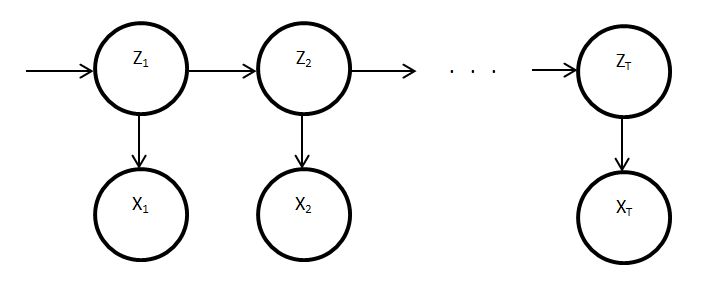
The model of appliances using HMMs can be extended to include such information. This requires the addition of a new sequence of observed variables, upon which the appliance states are conditionally dependent. This results in an input-output hidden Markov model as is shown below:

where:

• circles represent continuous variables, squares represent discrete variables
• shaded represent latent (hidden) variables, white represent observed variables
• a represents a sequence of an additional data source (e.g. time of day)
• z represents a Markov chain of appliance states
• x represents a sequence of appliance power readings
• T represents the number of time slices

By specifying the distribution of appliance states conditional upon the additional data source, the model can perform more accurate inference over appliance states without increasing the complexity of such inference. The probability of an assignment of values to the hidden variables can be calculated:

Explicit modelling of appliance duration

In the current model, the expected duration of each appliance's operation is modelled implicitly through the transition matrices. Although the transition probabilities are fixed for each time slice, they still determine the expected duration of an appliance when considering a sequence of observations. Consider an appliance with transition probabilities such that it will stay in the same state with probability 0.8 and change state with probability 0.2. We would expect the appliance to change state on average every 5 time slices, and such a sequence would be evaluated with a higher probability than one with state changes every 10 slices.

An alternative approach would be to model the probability of the next transition as conditionally dependent on the current state and its duration. The duration of the current state refers to the number of previous time slices during which the appliance's state has not changed. The graphical model stays unchanged, however the probability of an assignment of values to the hidden variables is now calculated:

where d at time slice n-1 refers to the duration of the current state.

This will complicate inference over the model, however such models have been successfully applied to many fields, including speech, human activity and hand writing recognition.

Steady-state analysis using hidden Markov models

So far we have used the sequence of power readings as the observed variables. Steady-state analysis is an alternative approach which aims to identify continuous states by the lack of change between consecutive power readings. HMMs can also be used for steady-state analysis by using the difference between consecutive power readings as the observed variable, instead of the power readings themselves. Inference over the HMM would remain the same, although the states in the HMM would no longer refer to appliance operating states. Instead, they would represent each possible transition to a new state in addition to a transition to the same state. The lattice diagram below shows the states of an HMM for steady-state analysis:

This above lattice diagram shows all the possible transitions between states. The lattice is fully connected between consecutive time slices, with the exception of consecutive turn on and turn off states. This is due to the fact that an appliance must first turn on before it can turn off and visa versa.

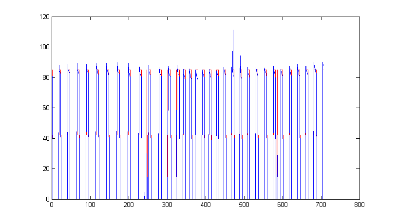
Each state is now responsible for a corresponding observation. For instance, the no change state would be expected to emit an observation close to 0, the turn on state might be expected to emit an observation of 50 while the turn off state would be expected to emit an observation of -50.

Conclusion

All three extension present improvements upon the existing appliance model, and should therefore lead to better appliance power disaggregation accuracy. However, I think the second method which uses semi-Markov models increases the complexity of inference for little gain in accuracy. However, the other two approaches provide significant advantages, in that the first allows predictions to be based on more data, while the second allows only a subset of appliances to be modelled. It should be possible to combine both of these two approaches, and therefore these will constitute a thorough investigation over the next few months.

9 Month Report: Using Hidden Markov Models for Non-intrusive Appliance Load Monitoring

Today I submitted my 9 month report:

Title: Using Hidden Markov Models for Non-intrusive Appliance Load Monitoring

Abstract: With the global problems of diminishing fossil fuel reserves and climate change comes the need to reduce energy consumption. One approach in the domestic sector is to improve consumer understanding of how much energy is consumed by each of their household appliances. This empowers consumers to make educated decisions on how they can change their lifestyle in an effort to reduce their energy consumption. This report investigates how total household energy consumption can be disaggregated into individual appliances using low granularity data collected from a single point of measurement, such as a smart meter. First, this work discusses how this problem can be solved using combinatorial optimisation. Second, a novel approach is introduced using hidden Markov models to model each appliance. We show through empirical evaluation that our implementation of the hidden Markov model approach outperforms the combinatorial optimisation method. Our future work is then outlined to show how we plan to better model domestic appliances and therefore improve the accuracy of our approach.

Using a single hidden Markov model to model multiple appliances

Previous posts have shown how a single appliance's states can be determined from its power readings using a hidden Markov model. This post shows how a single hidden Markov model can be used to determine the states of multiple appliances from their aggregate power readings.

Model definition

The combination of multiple latent Markov chains (representing appliance states) and a single observed variable (aggregate power readings) can be modelled as a factorial hidden Markov model:

A factorial hidden Markov model can actually be transformed to an equivalent standard HMM. Such a model would contain a single chain of latent variables, each of which has as many discrete states as the number of combinations of each appliance's states. For instance, for a FHMM with 3 latent chains of 2, 3 and 4 states each, the equivalent HMM will have 1 latent chain of 24 states. The standard HMM is shown below:

Learning

Before any inference can take place, the model parameters for the combined hidden Markov model must be specified:

• pi - the probability of each appliance state in time slice 1
• A - appliance transition probability matrix
• phi - emission density (probability density of observed variable given a hidden variable)

For training purposes, we assume to have training data for each individual appliance. The model parameters for each individual appliance can be learnt using the Expectation-Maximisation algorithm. The model parameters for each individual appliance must then be combined to a single set of model parameters for the combined hidden Markov model. The model parameters for the combined model are calculated:

• pi - the product of each combination of individual initial probability
• A - the product of each combination of transition probability
• phi - the sum of each combination of emission density

Once these model parameters have been calculated, the model is then ready to perform inference.

Inference

The Viterbi algorithm can be used to infer the most probable chain of latent variables in a HMM given a chain of observations. This is different to sequentially classifying variables according to their maximum probability. This is because the sequential classification method is unable to classify a state which is individually sub-optimal, but leads to a sequence of states which are jointly more probable. Because such classifications are not revisited sequential classification does not guarantee to find the jointly optimal sequence of states.

The complexity of the Viterbi algorithm is linear in the length of the Markov chain. However, its complexity is exponential in the number of appliances modelled. This is because the probability of each transition must be evaluated at each time slice. Since the variables correspond to each combination of all the appliance's states, the number of transitions is exponential in the number of appliances. This is acceptable for small numbers of appliances, but would become intractable for households containing many more than 20 appliances.

Calculating the optimal appliance state transitions for an observed data set - continued

This post extends the previous post, by applying the same technique to a multi-state appliance. The classification accuracy was tested using the power demand from a washing machine. The power demand for two cycles of a washing machine is shown below.

Each cycle consists of two similar states drawing approximately 1600 W, connected by an intermediate state drawing approximately 50 W. The intermediate state always connects two on states, and therefore the model should never classify transitions between the intermediate state and off states. This can be represented by the finite state machine below.

The HMM should capture such appliance behaviour. Therefore, it was set up such that the hidden variable has three possible states: 1 (off), 2 (intermediate) and 3 (on). The observed variable now represents a sample from this Gaussian mixture, and the Gaussian responsible for generating each sample is represented by the corresponding latent variable.

The model parameters pi (probabilities of first state), A (transition probabilities) and phi (emission densities) were set up:

• pi = [1 0 0] - The appliance will always be off at the start of the sequence
• A = [

             0.9,  0,     0.1
             0,     0.8,  0.2
             0.1,  0.1,  0.8
             ] - The appliance is most likely to stay in the same state, while transitions between off and intermediate are not possible

• phi = {mean: [2.5 56 1600], cov:[10 10 10]} - The distribution of the emissions of the Gaussian mixture

The transition matrix, A, models impossible state transitions as having probability 0. It also models highly probable transitions within states as close to 1.

After creating the HMM and setting the model parameters, the evidence can be entered into the inference engine. In this case, the evidence is the power demand shown by the graph at the top of this post. Once the evidence is entered, the Viterbi algorithm can be run to determine the optimal sequence of states responsible for generating the sequence of observations. The graph below shows a plot of the state sequence, where 1 = off, 2 = int, 3 = on.

Such a probabilistic approach to state classification has advantages over dividing the power demand using static boundaries. First, the approach is robust to noise, in that variations around a mean demand in the intermediate and on states do not detrimentally affect their classification. Second, samples taken during a transition are typically ignored if no probable transition exists. For instance, one or two samples are captured during the transition between the off and on states. Instead of classifying these as the intermediate state, these are assumed to be noise and correctly classified as the off state.

This approach allows information about the most probable transitions to built into the model given the sequential nature of observations. This is an extension to simply selecting the appliance state most likely to generate the observation.

I intend to investigate how this approach can be extended to multiple appliances in the near future.

Calculating the optimal appliance state transitions for an observed data set

As explained in previous posts, we can model the conditional probabilities of appliance states and aggregate power readings using a Markov chain of latent variables:

where:

• Zt - discrete latent variable at time t (appliance state)
• Xt - continuous observed variable at time t (power reading)

This model can be manually trained by specifying the model parameters:

• pi - probability density of z1 (probabilities of initial appliance states)
• A - appliance transition probability matrix
• phi - emission density (probability density of observed variable given a hidden variable)

The problem of non-intrusive appliance load monitoring can be formalised as:

Given a sequence of observed power readings, X, determine the optimal sequence of appliance states, Z, responsible for generating such a sequence.

The probability of a sequence of appliance states and power readings can be evaluated using:

As previously described, the optimal sequence of appliance states can be found using the Viterbi algorithm.

I have used the Bayes Net Toolbox for Matlab to model a single two-state appliance. The model is manually trained by specifying the model parameters pi, A and phi. It is then possible to sample realistic data of arbitrary length from the model. In addition, it possible to evaluate the probability of a sequence of appliance states and power readings. Therefore, the Viterbi algorithm can be used to find the optimal sequence of appliance states for an observed sequence of power readings. I have implemented the Viterbi algorithm and used it to calculate the optimal sequence of states for a fridge, given a sequence of the fridge's power readings. Below is a graph showing the fridge's power reading (blue) and the estimated appliance states (red), where 85 represents on and 0 represents off.

In this case of a single two-state appliance, this approach performs similarly to simply comparing the power samples, p, against a threshold, x, where p > x indicates the appliance is on, and off otherwise. However, using this probabilistic approach has advantages over such a heuristic approach. The threshold method would always estimate the appliance be on if the power reading is above a given value, and therefore treats the data as independent and identically distributed. Conversely, the probabilistic approach takes into account the appliance's previous state and the probability of it changing state, and therefore exploits the sequential nature of the data.

This method is easily extended to a single appliance with more than two states, an approach which I intend to explore in the near future. This method can also potentially be extended to many appliances with multiple states, an approach that I intend to explore in the more distant future.

Data simulation using concurrent independent Markov chains of latent variables

As explained in previous posts, we can model the conditional probabilities of appliance states and aggregate power readings using a Markov chain of latent variables:

where:

• Zt - discrete latent variable at time t (appliance state)
• Xt - continuous observed variable at time t (power reading)

This model can be manually trained by specifying the model parameters:

• pi - probability density of z1 (probabilities of initial appliance states)
• A - appliance transition probability matrix
• phi - emission density (probability density of observed variable given a hidden variable)

The model can then be used to simulate the states of an appliance and its power demand over time.

This is trivially extended to multiple appliances by using multiple concurrent Markov chains. However, this makes the assumption that appliance operations are independent of each other. Aggregate readings would be calculated by summing over each chain's observed variable for each time slice. Gaussian noise can be added to such a model using an additional Markov chain of latent variables, in which the latent variable is discrete and has only one state and the emission density represents the noise. This is equivalent to the factorial hidden Markov model below:

where:

• Zt (1...n) - discrete latent variable at time t (appliance state)
• Zt (0) - discrete latent variable at time t (meter noise source)
• Xt - continuous observed variable at time t (power reading)

Classification a single appliance's state using a hidden Markov model

The simplest scenario is one in which we wish to determine the state of a single two-state appliance, given its power demand. This can be represented as a hidden Markov model as follows:

where:

• Zt - hidden (latent) variable at time t (appliance state)
• Xt - observed variable at time t (power reading)

For a given set of observed variables, we can expand the possible chains of hidden variable states as a lattice diagram:

where:

• k - appliance state

It can be seen from this diagram that the number unique chains of hidden variables through this lattice scales exponentially with the length of the chain. However, the max-sum algorithm (called the Vertibi algorithm in this case) can be used to find the probability of the most likely chain, with complexity that grows only linearly with the length of the chain. The values of the most likely chain can then be found by backtracking through the chain starting from the final time slice of the most likely chain.

The Viterbi algorithm involves calculating the joint probability of a chain of observed and hidden variables, given by:

where:

• X - set of observed variables
• Z - set of hidden variables
• theta = {pi, A, phi} - model parameters
• pi - probability density of z1
• A - appliance transition probability matrix
• phi - emission density (probability density of observed variable given a hidden variable)
• N - number of time slices

The model parameters parameters can be learnt from the set of observed variables using the Expectation-Maximisation algorithm. However, we may want to introduce a prior belief over some parameters, or even fix some parameters. For example, we might know the state of the appliance at the start of the chain, and can therefore fix pi. We might also know the parameters governing the emission density, and if we assume the observations are normally distributed we might want to fix the mean and variance parameters of the Gaussian function.

Although this model can represent appliances with more than two states, it is unclear how tractable the EM algorithm will be for a factorial hidden Markov model. One solution would be to model the multiple Markov chains as a single Markov chain, whose number of states is equal to the number of combinations of appliance states. However, the complexity of such a model is then exponential in the number of appliances. It is worth noting that we can prune the number of possible transitions based on the assumption that only one appliance can change state between two consecutive time slices, which is a practical assumption assuming a small time interval between time slices. A solution to solving this might be to use sampling methods.

NIALM as a factorial hidden Markov model

After considering various heuristic approaches towards NIALM, it is clear that a more principled probabilistic approach is required. The approach would need to recognise that premise-level power readings are sequentially drawn from a continuous time series, and are not independent of each other. In fact, intuition tells us that in general appliances are far more likely to stay in their current state, and that state changes are comparatively rare. NIALM can also be considered as an online-learning problem, in which disaggregation must occur after each individual premise-level power value has been received. These two assumptions map directly on to the modelling of such a problem as a factorial hidden Markov model.

In a factorial hidden Markov model, there are multiple independent chains of hidden variables, which in this case are the current operating state of each appliance. At each time slice, there is also an observed variable conditional on the states of all of the corresponding hidden variables, which in the case is the premise-level power value. Below is a diagram of a factorial hidden Markov model.

where:

• Z - hidden (latent) variable, subscript - time slice, superscript - variable number
• X - observed variable, subscript, time slice

NIALM solutions are interested in evaluating the state of appliances, and given a look-up table of appliance state power values, can therefore evaluate the power of each appliance at each time slice. We are therefore interested in modelling the probability of an appliance being in a certain state, given the appliance's state in the previous time slice and the observed variable for that time slice:

This is an approach I will be investigating over the following weeks, after reading up on the relevant theory on sequential data and expectation-maximisation.

NIALM as a combinatorial optimisation problem - continued

As previously discussed, appliance loads can be disaggregated from premise-level power readings by the minimisation of a function f at each time slice:

where:

• Pagg - premise-level aggregate power
• N - number of appliances
• I - vector of appliance binary indicators (1 if appliance is on, 0 otherwise)
• P - vector of appliance power when appliance is on

Two commonly cited disadvantages of this approach is how its accuracy would decrease with the number of appliances and level of noise. However, no research has been published investigating the situations in which this approach performs sufficiently accurately. I have tested this approach using simulated data for 24 time slices, relating to one reading per hour over the course of a day. Below are tests evaluating the performance of this approach as the number of appliances is increased and as the noise in the data is increased.

Increasing numbers of appliances

Below shows a graph of this approach's true positive rate (TPR) and false positive rate (FPR) for increasing numbers of appliances, n. No noise was introduced over the simulated data set.

We can see that this approach performs very accurately from n = 1 to roughly n = 10. However, for n > 10 the TPR rapidly decays towards 0.5, while the FPR increases towards 0.25. This approach is clearly only useful for small n (roughly n < 20). However, it might be interesting to evaluate the performance of this method given only a small subset of appliances and the premise-level aggregate power. The appliances should be chosen such that they are the most power hungry appliances.

Increasing noise

To investigate how the accuracy of this approach is affected by noise, Gaussian noise was added to the premise-level power readings of the form:

where:

• N - Gaussian distribution
• x - Noisy premise-level aggregate
• Pagg - actual premise-level aggregate
• c - noise level

Below shows a graph of this approach's true positive rate (TPR) and false positive rate (FPR) for increasing noise in the aggregate power reading, c.

We can see that instantly after introducing some noise, the TPR rate drops to roughly 0.7 for Gaussian noise of standard deviation just 0.1% of the aggregate power level. It is clear that this approach is not robust to even small levels of noise in the premise-level aggregate power readings, as would be likely in a realistic setting.

Extensions

Two extensions are discussed below which could increase the accuracy of this approach.

First, the assumption that an appliance has only one state for which it can draw power can be relaxed. Instead, we allow appliances to operate in one of a number of K states, each of which has a unique power value. The appliance state indicator variable would therefore be a binary vector taking the form of a 1-of-K coding scheme, such that:

and

The optimal appliance combination would therefore be given by minimising the function f at each time slice:

Second, the assumption that appliance states at each time slice are independent of each other can be relaxed. This allows us to take into account information of known appliance lengths in the form of constraints, e.g. 10 minutes < fridge_cycle_duration < 20 minutes. However, this would significantly increase the complexity of the optimisation problem by including the additional time dimension.

NIALM as a combinatorial optimisation problem

NIALM can be formulated as a combinatorial optimisation problem as follows:

For each time instant, minimise the function f:

where:

• Pagg - household aggregate power
• N - number of appliances
• I - vector of appliance binary indicators (1 if appliance is on, 0 otherwise)
• P - vector of appliance power when appliance is on

This approach was first proposed by Hart, as explained in the 1992 seminal paper on NIALM. Hart asserts that this is an NP-complete "weighted set" problem, and mentions that the number of combinations of 'on' appliances scales exponentially with the number of appliances. However, despite its computational difficulty, the optimal solution can be found within seconds for a realistic number of appliances, e.g. 30.

I have recently been investigating the performance of this technique using simulated data. 24 hours worth of truth data was generated using 30 appliance profiles, each with realistic power demands and usage patterns. The true household aggregate was calculated by summing the power consumed by each device at that time instant. No noise was added on appliance nor household level.

I have been investigating how the performance of this technique decays as the number of appliances in the household increases. The optimisation function was applied at 1 hour intervals to 24 hours of data, and the accuracy was calculated as the average fraction of correct classifications.

Below is a graph showing the accuracy of this technique for the number of appliances in the house.

The technique is very accurate when there is less than 10 appliances in the household. Although the accuracy starts to drop rapidly, if seems to converge around 0.5 or 0.6. However, further tests of large numbers of appliances are necessary to prove this.

Obvious future work is to investigate how the performance of this approach decays with the introduction of appliance and aggregate level noise to the data.

My electricity consumption separated into lighting and appliances

I've recently been monitoring my electricity consumption using two AlertMe clamps round my household aggregate and lighting circuits. The graph below shows the power draw for Sunday 20.03.2011.

It is interesting to note how easy it is to recognise some specific appliances.

• Fridge - 35-40 cycles throughout the day. The fridge's square power draw is clearly visible throughout the night, and at various points throughout the day. However, it is less obvious in the evening when many other appliances are operating.
• Kettle - 10.00, 13.00, 17.30, 19.00. The kettle is distinguishable by its power draw of 2.5kW and its short duration for 2-3 minutes.
• Washing machine - 13.00, 15.30. The washing machine has an alternating power draw between 600W and 0W for its 1 hour cycle duration. However, it also has a solid power draw of 2kW for about 20 minutes.
• Oven - 18.30-19.30, 21.30-22.30. The oven's temperature is regulated by a thermostat so its power draw predictably alternates between 0W and 2kW. However, there is a period while it initially heats up to temperature when it is on continuously. For the first use the temperature was set to 170 degrees, while for the second use it was set to 110 degrees. This is reflected by the duration between 'on' cycles, similar to Alex's fridge's behaviour.

It is also interesting to analyse the lighting circuit's power draw. Since each light only has two states, 'on' and 'off', techniques such as steady-state analysis or combinatorial optimisation would work well here.