9 Month Report: Using Hidden Markov Models for Non-intrusive Appliance Load Monitoring

Today I submitted my 9 month report:

Title: Using Hidden Markov Models for Non-intrusive Appliance Load Monitoring

Abstract: With the global problems of diminishing fossil fuel reserves and climate change comes the need to reduce energy consumption. One approach in the domestic sector is to improve consumer understanding of how much energy is consumed by each of their household appliances. This empowers consumers to make educated decisions on how they can change their lifestyle in an effort to reduce their energy consumption. This report investigates how total household energy consumption can be disaggregated into individual appliances using low granularity data collected from a single point of measurement, such as a smart meter. First, this work discusses how this problem can be solved using combinatorial optimisation. Second, a novel approach is introduced using hidden Markov models to model each appliance. We show through empirical evaluation that our implementation of the hidden Markov model approach outperforms the combinatorial optimisation method. Our future work is then outlined to show how we plan to better model domestic appliances and therefore improve the accuracy of our approach.

Using a single hidden Markov model to model multiple appliances

Previous posts have shown how a single appliance's states can be determined from its power readings using a hidden Markov model. This post shows how a single hidden Markov model can be used to determine the states of multiple appliances from their aggregate power readings.

Model definition

The combination of multiple latent Markov chains (representing appliance states) and a single observed variable (aggregate power readings) can be modelled as a factorial hidden Markov model:

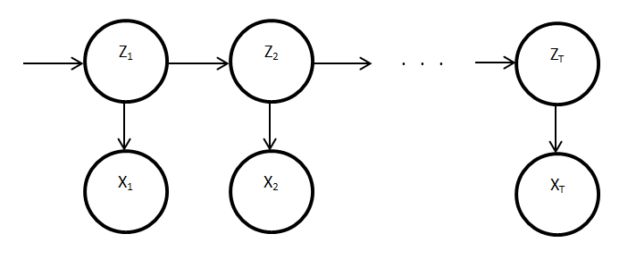
A factorial hidden Markov model can actually be transformed to an equivalent standard HMM. Such a model would contain a single chain of latent variables, each of which has as many discrete states as the number of combinations of each appliance's states. For instance, for a FHMM with 3 latent chains of 2, 3 and 4 states each, the equivalent HMM will have 1 latent chain of 24 states. The standard HMM is shown below:

Learning

Before any inference can take place, the model parameters for the combined hidden Markov model must be specified:

• pi - the probability of each appliance state in time slice 1
• A - appliance transition probability matrix
• phi - emission density (probability density of observed variable given a hidden variable)

For training purposes, we assume to have training data for each individual appliance. The model parameters for each individual appliance can be learnt using the Expectation-Maximisation algorithm. The model parameters for each individual appliance must then be combined to a single set of model parameters for the combined hidden Markov model. The model parameters for the combined model are calculated:

• pi - the product of each combination of individual initial probability
• A - the product of each combination of transition probability
• phi - the sum of each combination of emission density

Once these model parameters have been calculated, the model is then ready to perform inference.

Inference

The Viterbi algorithm can be used to infer the most probable chain of latent variables in a HMM given a chain of observations. This is different to sequentially classifying variables according to their maximum probability. This is because the sequential classification method is unable to classify a state which is individually sub-optimal, but leads to a sequence of states which are jointly more probable. Because such classifications are not revisited sequential classification does not guarantee to find the jointly optimal sequence of states.

The complexity of the Viterbi algorithm is linear in the length of the Markov chain. However, its complexity is exponential in the number of appliances modelled. This is because the probability of each transition must be evaluated at each time slice. Since the variables correspond to each combination of all the appliance's states, the number of transitions is exponential in the number of appliances. This is acceptable for small numbers of appliances, but would become intractable for households containing many more than 20 appliances.

Calculating the optimal appliance state transitions for an observed data set - continued

This post extends the previous post, by applying the same technique to a multi-state appliance. The classification accuracy was tested using the power demand from a washing machine. The power demand for two cycles of a washing machine is shown below.

Each cycle consists of two similar states drawing approximately 1600 W, connected by an intermediate state drawing approximately 50 W. The intermediate state always connects two on states, and therefore the model should never classify transitions between the intermediate state and off states. This can be represented by the finite state machine below.

The HMM should capture such appliance behaviour. Therefore, it was set up such that the hidden variable has three possible states: 1 (off), 2 (intermediate) and 3 (on). The observed variable now represents a sample from this Gaussian mixture, and the Gaussian responsible for generating each sample is represented by the corresponding latent variable.

The model parameters pi (probabilities of first state), A (transition probabilities) and phi (emission densities) were set up:

• pi = [1 0 0] - The appliance will always be off at the start of the sequence
• A = [

             0.9,  0,     0.1
             0,     0.8,  0.2
             0.1,  0.1,  0.8
             ] - The appliance is most likely to stay in the same state, while transitions between off and intermediate are not possible

• phi = {mean: [2.5 56 1600], cov:[10 10 10]} - The distribution of the emissions of the Gaussian mixture

The transition matrix, A, models impossible state transitions as having probability 0. It also models highly probable transitions within states as close to 1.

After creating the HMM and setting the model parameters, the evidence can be entered into the inference engine. In this case, the evidence is the power demand shown by the graph at the top of this post. Once the evidence is entered, the Viterbi algorithm can be run to determine the optimal sequence of states responsible for generating the sequence of observations. The graph below shows a plot of the state sequence, where 1 = off, 2 = int, 3 = on.

Such a probabilistic approach to state classification has advantages over dividing the power demand using static boundaries. First, the approach is robust to noise, in that variations around a mean demand in the intermediate and on states do not detrimentally affect their classification. Second, samples taken during a transition are typically ignored if no probable transition exists. For instance, one or two samples are captured during the transition between the off and on states. Instead of classifying these as the intermediate state, these are assumed to be noise and correctly classified as the off state.

This approach allows information about the most probable transitions to built into the model given the sequential nature of observations. This is an extension to simply selecting the appliance state most likely to generate the observation.

I intend to investigate how this approach can be extended to multiple appliances in the near future.