My electricity consumption separated into lighting and appliances

I've recently been monitoring my electricity consumption using two AlertMe clamps round my household aggregate and lighting circuits. The graph below shows the power draw for Sunday 20.03.2011.

It is interesting to note how easy it is to recognise some specific appliances.

• Fridge - 35-40 cycles throughout the day. The fridge's square power draw is clearly visible throughout the night, and at various points throughout the day. However, it is less obvious in the evening when many other appliances are operating.
• Kettle - 10.00, 13.00, 17.30, 19.00. The kettle is distinguishable by its power draw of 2.5kW and its short duration for 2-3 minutes.
• Washing machine - 13.00, 15.30. The washing machine has an alternating power draw between 600W and 0W for its 1 hour cycle duration. However, it also has a solid power draw of 2kW for about 20 minutes.
• Oven - 18.30-19.30, 21.30-22.30. The oven's temperature is regulated by a thermostat so its power draw predictably alternates between 0W and 2kW. However, there is a period while it initially heats up to temperature when it is on continuously. For the first use the temperature was set to 170 degrees, while for the second use it was set to 110 degrees. This is reflected by the duration between 'on' cycles, similar to Alex's fridge's behaviour.

It is also interesting to analyse the lighting circuit's power draw. Since each light only has two states, 'on' and 'off', techniques such as steady-state analysis or combinatorial optimisation would work well here.

Bayesian modelling of appliance detections using smoothness metrics and cycle frequency

Previously, I discussed the use of Bayesian modelling for appliance signature matching. Following Bayes rule, the posterior is proportional to the product of the prior and the evidence:

where:

• X = candidate appliance cycle corresponding to actual appliance cycle
• t = time between known previous appliance cycle and candidate appliance cycle

The prior, P(X), will be calculated using a combination of smoothness metrics. The evidence, P(t|X), will be calculated using the known probability distribution of times between appliance cycles. These are explained respectively below.

Prior: P(X)

So far, I have proposed three metrics for assigning a confidence value to a possible appliance cycle. When defining them, I'll use the following notation:

• P = Aggregate power
• A = Appliance power
• Q = P - A
• t = time instant from 1 to T

1DERIV:
Difference between the sum over the first derivative of the aggregate power and the first derivative of the aggregate-appliance power:

2DERIV:
Difference between the sum over the second derivative of the aggregate power and the second derivative of the aggregate-appliance power:

ENERGYRATIO:
Ratio of the energy consumed by the appliance during its cycle and the energy consumed by all other appliance's during the cycle:

where:

• a = time instant of cycle start
• b = time instant of cycle end

Evidence: P(t|X)


We know the probability distribution of the time between appliance cycles. This is shown by the histogram below:

This can be modelled using a normal distribution of mean and standard deviation calculated from this data set. This model will be used to calculate the evidence probability.

Posterior: P(X|T)


I have calculated the posterior using two combinations of smoothness metrics to form the prior:

1. threshold(1DERIV) * 2DERIV
2. threshold(1DERIV) * ENERGYRATIO

In both cases, the 1DERIV metric has been used to calculate whether subtracting the appliance signature had smoothed the aggregate power array. A threshold was applied to these smoothness values to produce a list of candidates for which the subtraction increased the smoothness of the array. Next, the candidates were multiplied by a confidence metric. In the first case the 2DERIV metric was used, and in the second case the ENERGYRATIO metric was used.

Given a known appliance cycle and a number of candidates for the immediately following cycle, the posterior probability for each candidate cycle was calculated. The maximum likelihood candidate cycle was selected as a correct cycle and the process was repeated sequentially for the remaining cycles.

The two plots below show the estimated fridge cycles (blue) against actual fridge cycles (red).

1. threshold(1DERIV) * 2DERIV

2. threshold(1DERIV) * ENERGYRATIO

Both estimations worked well, correctly detecting 23 and 24 cycles respectively, out of 31 actual cycles. Each method actually only generated 30 positives, of which 7 and 6 were false positives respectively. There was a common interval in which neither approach generated a true or false positive, occurring at a time when the off duration was at a minimum. The use of a model with an off duration that varies over time might increase the performance of both approaches here.

In addition, it is interesting to note that there are some areas where approach 1 outperforms approach 2, and other areas where approach 2 outperforms approach 1. This is encouraging, as it could mean that the two approaches are complementary. I investigated using a third approach in which the confidence metric was the product of 2DERIV and ENERGYRATIO, although the result was less accurate than either individual approach.

More smoothness metrics

Recently I've been looking at whether subtracting an appliance's known signature from the aggregate demand increases the smoothness of the curve. The success of such an approach is clearly dependant on what smoothness metric is used. I've already looked at the sum of the changes in power:

This is equivalent to taking the first derivative if the power values, because the denominator, dt, is always 1.

However, recently I've been troubled by the way this metric indicates an optimal match for the five graphs shown below. They are all possible combinations of the fridge's signature (red) with other appliances (blue). The vertical corresponds to power (W) while the horizontal corresponds to time (minutes).

However, we'd prefer the metric to return an optimal match for graphs A-D, and a sub-optimal match for graph E. This is because it is far less likely that another appliance of the same duration as the fridge will coincide with both the fridge's 'on' and 'off' transitions.

In an effort to quantify this, I realised that subtracting the fridge's signature reduces the number corners in graphs A-D, but not in E. Since a corner corresponds to a change in gradient, the second derivative of P might be a useful metric for smoothness:

The absolute value of the second derivative of P with respect to t will produce a positive value corresponding to each corner, and 0 otherwise. Therefore, the number non-zero values produced by this function is a measure of the noisiness of a curve. Taking the reciprocal provides us with the desired smoothness metric.

Weekly supervisor meeting

Following today's meeting, there are two approaches I want to investigate further this week:

1. Bayesian modelling of appliance detections using smoothness and confidence levels
2. Time instant combinatorial optimisation

Bayesian modelling of fridge detections using smoothness and confidence levels

I'm going start by applying a threshold to the smoothness values calculate after subtracting the fridge's signature from the aggregate signal at each possible interval. This will look something like this:

For each value above the threshold, I will lookup the confidence value as is given by the confidence plot:

So, let:

X = smoothness peak corresponds to fridge cycle

t = time since last cycle

This confidence value will form the prior probability that the fridge is operating during this time period, X

We can form a likelihood too given the distribution of time between cycles, t

Therefore, using Bayes:

P(X | t) proportional to P(t | X) * P(X)

Therefore, the probability of each smoothness peak corresponding to the next fridge's cycle can be calculated, given the previous cycle. The optimum cycle will be then be selected using maximum likelihood. This process will be repeated sequentially for each cycle over the course of the day.

I believe this approach is similar to the hidden Markov model of this problem, although I haven't read much into the underlying theory of this area yet.

Time instant combinatorial optimisation

This was explained in detail in the previous post. For convenience, I've repeated it below.

Minimise the error function f:

f =

where:

• t is a time instant in the range 1...T
• n is an appliance the range 1...N
• P agg is the aggregate power
• I is a vector of binary values indicating the state of an appliance. Only one value will be non-zero
• P is a vector of continuous values indicating the power values for each state of an appliance

This approach has been frequently mentioned and dismissed within the NALM literature (initially by Hart in 1992) for a number of valid reasons. I want to investigate how well this works for increasingly complex data:

1. Small number of appliances (5) for which the complete set of states for all appliances is known
2. As in 1 but with some noise
3. As in 1 but for a realistic number of appliances (20)
4. As in 3 but with an incomplete set of appliances

Discussion of machine learning approaches with Sid

I've had some lengthy discussions with Sid about some machine learning approaches which could be applied to the field of NALM. He advised me not to get stuck in to one method, but investigate as much as I can. In addition, he also advised me to be careful not to unnecessarily add complexity to approaches. It is still a contribution to implement simple techniques which other academics had previously discarded, even if they are only used as benchmarks. Following this I will explore the following techniques:

Time instant combinatorial optimisation


Minimise the error function f:

f =

where:

• t is a time instant in the range 1...T
• n is an appliance the range 1...N
• P agg is the aggregate power
• I is a vector of binary values indicating the state of an appliance. Only one value will be non-zero
• P is a vector of continuous values indicating the power values for each state of an appliance

This approach has been frequently mentioned and dismissed within the NALM literature (initially by Hart in 1992) for a number of valid reasons. I want to investigate how well this works for increasingly complex data:

1. Small number of appliances (5) for which the complete set of states for all appliances is known
2. As in 1 but with some noise
3. As in 1 but for a realistic number of appliances (20)
4. As in 3 but with an incomplete set of appliances

Time interval combinatorial optimisation


Extend the previous optimisation problem from a 1-dimensional to a 2-dimensional problem. This is achieved by minimising the error function over an interval of time, instead of for each time instant. The following constraints would be included for each appliance:

• Appliance operation model (possibility and probability of transitions between states)
• Length of state (minimum and maximum duration of states)

Factorial hidden Markov models


Represent the problem as a factorial hidden Markov model, where each observation (aggregate power reading) is a function of many state variables (appliance power values). This model is particularly suitable as the observations and state variables are sequential samples over time, and therefore depend on previous samples. If this dependence factorises along the chain of dependence, we can say that the value of a state variable at time t depends entirely on the the value of the same state variable at time t-1.

Assigning confidence to appliance detections

This post follows up on a previous post on using smoothness to detect appliances. The problem with this method is the large number of false positives it generates in addition to correct appliance matches. The appliances for which this method generates the most false positives are the appliances with low power consumption relative to the aggregate consumption. This post describes the assignment of confidence values to the appliance detections in an attempt to distinguish between true appliance detections and false positives.

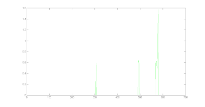
Below is a plot of the household aggregate power demand (W) and sub-metered appliances over a 24-hour period. The household aggregate is shown in black, the fridge in blue, the washing machine in green and the dishwasher in red.

As before, each appliance's signature was subtracted from the aggregate demand in turn, and the smoothness of the resulting plot was calculated. The fridge, washing machine and dishwasher's smoothness plots are shown below. In addition, we want to assign confidence to each of these appliance detections. This confidence value can be approximated using the ratio of energy consumed by the appliance in a typical cycle to energy consumed by other appliances during that time period. We define a confidence function such that:

if aggregate - signature > 0 for all power values

confidence(smoothness value) = SUM(signature_energy) / SUM(aggregate_energy - signature_energy)

else

confidence(smoothness value) = 0

endif

The if condition represents the possible interval heuristic as explained in a previous post. In this case it has been extended to two dimensions, in that a two dimensional power signature is used as opposed to a single value 'on' power value. This ensures that if the aggregate_energy - signature_energy has any value below 0, a confidence of 0 will be given.

The smoothness and confidence for the fridge, washing machine and dishwasher are shown below.

Fridge:

Smoothness:

Confidence:

This shows that the detections overnight have been assigned a higher confidence than most of the detections during the day, successfully distinguishing the clear positives from the false and unsure positives. In addition, two detections during the day when there were few other appliances operating were assigned a high confidence value. This approach has worked very well for the fridge data.

Washing machine:

Smoothness:
Confidence:

This confidence plot is a complete contrast to the fridge's plot. In this case, there are only three instances where the signature can be subtracted from the aggregate signal, each with a fair confidence level. However, the highest confidence is assigned to the third match, while only the first match corresponds to an actual cycle of the washing machine. The reason for this is the first two matches have much higher power peaks than the washing machine would cause, while the shape of the third detection matches the signature well.

Dishwasher:

Smoothness:

Confidence:

Similar to the washing machine's confidence plot, this provides very little data. A high confidence is assigned to the first match found by the smoothness appliance detector. However, no confidence value is assigned to the second correct detection. This is due to an inaccuracy in the power data collected by either the aggregate or washing machine Plogg.

As can be seen on the graph at the top of this post, there is a time instant at which the washing machine Plogg records a higher power value than the household aggregate. This should not be possible, as the household aggregate should include the washing machine in addition to all other electrical appliances. This inaccuracy most likely occurred due to a slight discrepancy between the time at which the Ploggs record a certain data value. I assume this was caused by the washing machine momentarily dipping its power draw as it was sampled by the household aggregate Plogg, before increasing its power draw and being sampled by the washing machine Plogg.

Conclusions:

This confidence metric works very well for appliances whose signature is relatively small compared to the aggregate profile. However, the confidence metric adds little information for appliance's whose signature is relatively large compared to the aggregate profile. This is because it is only applicable when the appliance's signature can be subtracted from the household aggregate, and therefore mimicking the 'possible interval' heuristic.

Load Signature Study—Part II: Disaggregation Framework, Simulation, and Applications

Liang J, Ng SKK, Kendall G, Cheng JWM. Load Signature Study - Part II: Disaggregation Framework, Simulation, and Applications. IEEE Transactions on Power Delivery. 2010;25(2):561-569.

This paper reports an evaluation of the disaggregation methods proposed in part I using the previously described accuracy metrics. The evaluation is based on data created through simulation of a household's aggregate demand. The simulation triggers appliance 'on' and 'off' events given a database of appliance signatures and usage likelihoods. The authors conclude that committee decision mechanisms (CDM) outperform single-feature and single algorithm disaggregation methods, with the Maximum Likelihood Estimation CDM performing the best. The authors also note that CDMs are less sensitive to appliance signature noise and aggregate noise.

The use of simulation to generate data upon which the algorithms are evaluated is very interesting. While a range of datasets can be generated far more easily than real-time monitoring, there are also a number of disadvantages. Primarily, any information based on human behaviour, e.g. appliance usage frequency, is lost in the simulation. In addition, any assumptions upon which the simulation is based can cause unrealistic data to be generated. In this paper, the simulation considers appliances whose signatures consist of an 'on' event, followed by a period of constant consumption and ending with an 'end' event. This 'on'-'off' model clearly fails to capture behaviour of appliances with multiple steady states, slow gradual transitions or continuously varying signatures. Furthermore, the simulation assumes only one appliance switch event will occur between samples. This is also an unrealistic assumption, oversimplifying the required disaggregation methods.

Despite the drawbacks of using simulation to evaluate the accuracy of the proposed disaggregation methods, the conclusions related to CDMs are still strong. CDMs are effective techniques to combine feature extraction and classification methods, will be applicable to most NALM approaches.