Top 10 papers for Non-Intrusive Appliance Load Monitoring (NIALM) - updated for 2011

Update: Top papers of 2012

About a year ago I posted a short list of some of the most useful papers for NIALM. Since then I have learnt a lot, found much more material and read many newly published papers. This post is intended as an update to the original list, containing what I now believe to be the most relevant and useful academic papers. Below is my top 10 papers for NIALM (in alphabetical order). Any comments and discussions are welcome!

• Berges ME, Goldman E, Matthews HS, Soibelman L. Enhancing Electricity Audits in Residential Buildings with Nonintrusive Load Monitoring. Journal of Industrial Ecology. 2010;14(5):844-858.
• This article provides an up-to-date overview of the practicalities of NIALM. Since many approaches require a specific monitoring device, it is useful to understand the range of hardware available and their associated costs. The authors relate the capabilities of such hardware to the potential for NIALM, including an overview of general appliance behaviour and their power demands.
• Chang H-H, Lin C-L, Lee J-K. Load identification in nonintrusive load monitoring using steady-state and turn-on transient energy algorithms. In: International Conference on Computer Supported Cooperative Work in Design.; 2010:27-32.
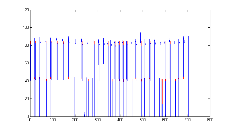
• This paper combines steady-state and transient-state NIALM approaches with strong classification methods from the field of machine learning. The authors use a trained neural network as the disaggregation decision engine based on the extracted features. It is clear from the paper that the use of transient energy can project previously indistinguishable inputs into unique feature space.
• Hart GW. Nonintrusive appliance load monitoring. Proceedings of the IEEE. 1992;80(12):1870-1891.
• This is the seminal work by Hart which defines the field of NIALM. The paper provides insight into the aims and applications of such technology, in addition to summarising both his own and other related work in the late 80s and early 90s. Hart explains the intuition behind many approaches to NIALM, including his 'total load model' (also known as integer programming or combinatorial optimisation) and 'appliance model' (which has since been extended using HMMs). Finally, the paper gives an unbiased evaluation of the realistic potential and limitations for the field.
• Kim H, Marwah M, Arlitt MF, Lyon G, Han J. Unsupervised Disaggregation of Low Frequency Power Measurements. In: The 11th SIAM International Conference on Data Mining. Mesa, Arizona; 2011:747-758.
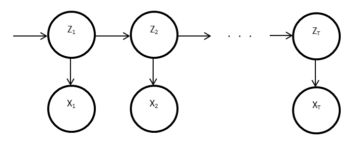
• This paper describes how Factorial HMMs (FHMM) from the machine learning domain can be used for NIALM. The authors cover the tractability of both training and inference over such models. Two extensions of the basic FHMM are described and evaluated; the use of additional data sources (e.g. time of day) and the dependencies between appliances (PC and monitor).
• Kolter JZ, Johnson MJ. REDD : A Public Data Set for Energy Disaggregation Research. In: Workshop on Data Mining Applications in Sustainability (SIGKDD). San Diego, CA; 2011:1-6.
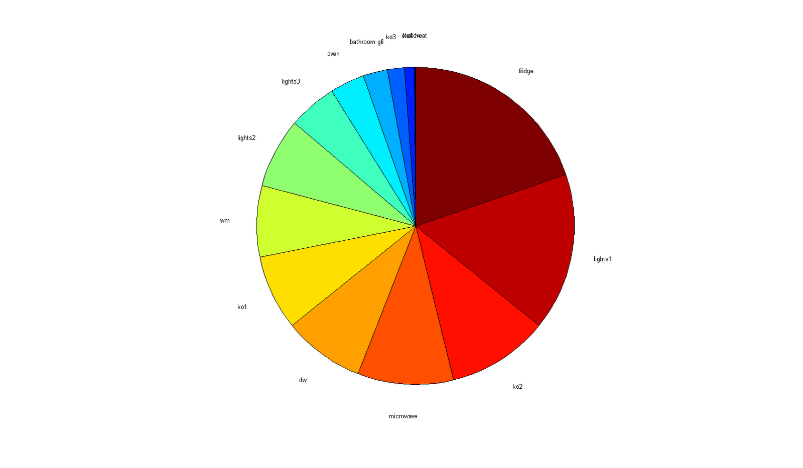
• This paper describes a recently published public data set for evaluating NIALM methods. This tackles the issue that, generally, energy disaggregation approaches are evaluated on different data sets, making direct performance comparison impossible. The data collected includes energy monitors at premises-level, circuit-level and appliance-level in 6 homes in the US. However, only premises-level data in kHz range and circuit-level data in Hz range have been realised in v1.0.
• Laughman C, Lee K, Cox R, et al. Power signature analysis. IEEE Power and Energy Magazine. 2003;1(2):56-63.
• This article provides a high level overview of the state of the art at the time of publishing. The approaches discussed include those applicable to high granularity data, such as harmonic and transient analysis, in addition to steady-state disaggregation methods. Finally, some intuition is given into how appliances with a continuously varying power draw can be disaggregated.
• Liang J, Ng S, Kendall G, Cheng J. Load Signature Study - Part I: Basic Concept, Structure, and Methodology. IEEE Transactions on Power Delivery. 2010;25(2):551-560.
• The first part of this pair of papers gives an in-depth and up-to-date discussion of the various approaches to NIALM. The authors also provide a useful description of how multiple approaches can be combined to give a single, more accurate classification. Finally, an evaluation of the many accuracy metrics which have been used is also given.
• Liang J, Ng SKK, Kendall G, Cheng JWM. Load Signature Study - Part II: Disaggregation Framework, Simulation, and Applications. IEEE Transactions on Power Delivery. 2010;25(2):561-569.
• The second part of this pair of papers gives a detailed description of a household simulator that would generate data that could be used to test NIALM algorithms. This allowed the authors to analyse the effect of many different situations, such as noise, concentration of appliance events, the impact of simultaneously operating appliances and the impact of similar appliances. The simulations confirm the first paper's proposal that the fusion of NIALM techniques can improve the disaggregation performance.
• Norford LK, Leeb SB. Non-intrusive electrical load monitoring in commercial buildings based on steady-state and transient load-detection algorithms. Energy and Buildings. 1996;24(1):51-64.
• This article gives a description of how NIALM techniques successful in domestic settings can be extended of commercial buildings. Interestingly, commercial buildings do not only present a new set of appliances, but also bring new applications to the field, such as fault detection. The authors discuss the performance of state-of-the-art steady-state and transient-state disaggregation methods at the time of publishing.
• Zeifman M, Roth K. Nonintrusive appliance load monitoring: Review and outlook. IEEE Transactions on Consumer Electronics. 2011;57(1):76-84.
• This paper is focussed entirely on giving a description and critique of all techniques applied within the NIALM field over the past 25 years. The range of approaches identified by the authors make this paper very useful when viewing the field as a whole. Accuracy metrics are also discussed, with the authors concluding that there is no agreed metric on which disaggregation performance should be assessed.

The Reference Energy Disaggregation Data Set

Accurately comparing the performance of energy disaggregation (Non-intrusive Appliance Load Monitoring) methods is almost impossible unless the same test data is used. For this reason, a team at MIT have built The Reference Energy Disaggregation Data Set (REDD). A few weeks ago, an initial (v1.0) snapshot of this data set was released for use in academic work. The paper describing the equipment used for data collection is:

Kolter JZ, Johnson MJ. REDD : A Public Data Set for Energy Disaggregation Research. In: Workshop on Data Mining Applications in Sustainability (SIGKDD). San Diego, CA; 2011

The dataset contains data for 6 houses. For each house:

• The current and voltage of the two mains circuits are monitored at 15kHz. This is also available for download as power readings down sampled to 1Hz
• The power of each circuit in the home is also monitored to a frequency of 1 reading every 3-4 seconds. Each house contains 11-26 circuits, with large appliances often operating on their own dedicated circuit
• The power drawn by individual appliances is also being monitored, although not enough data had been collected to warrant its release in v1.0

Collecting energy consumption data is a time consuming and expensive process. The lack of available data about appliance behaviour and energy consumption often limits the understanding necessary to design energy disaggregation methods. Through the study of this dataset, I hope to provide some insight into how the energy is consumed in the home and how energy disaggregation methods can take advantage of this.

Energy Breakdown

The aim of energy disaggregation methods is often to maximise the disaggregation accuracy, or minimise the difference between the predicted and actual energy consumption of each appliance. Therefore, the penalty for not recognising an appliance has consumed any energy increases with the energy consumption of the appliance. Consequently, it is more important for energy disaggregation methods to be able to disaggregate an appliance which consumes a high amount of energy than one that consumes a low amount of energy. So which appliances are most important? The figure below shows the relative contributions of each household circuit for house 1 of REDD.

Energy breakdown by circuit of house 1

The above figure shows that just 7 circuits collectively contribute over 75% of the house's total energy consumption. Admittedly, not all circuits contain a single appliance, although I doubt any circuit contains more than a handful of appliances. I'm a little surprised that the fridge comes out as the highest energy consumer, but I don't think it's unusual that it would contribute a fair portion of a house's energy consumption.

Appliance Behaviour

In order to disaggregate a household's energy consumption into the contributing appliances, it is often necessary to build models of such appliances. Analysing the power demand of each appliance is often a good place to start to decide what information such a model should contain. Since the fridge came out as the highest consumer, I've chosen to take a closer look the fridge's power demand in 5 of the REDD houses. Below is a plot of the power demand over a 45 minute period.

Almost all fridges have a different power demand, duration of use and periodicity. However, interestingly, they all share an identical model of usage, in that they all exhibit similar cyclic behaviour. For each fridge, the cycle begins with a single increase in power, which gradually decreases during the cycle and finally ends sharply. Although not ideal, this is encouraging for the purpose of general appliance models. Such a general model of fridges could be built, and would only need to be tweaked in order to match a specific fridge's signature.

Plan for refinement of appliance model

At this stage, there are three potential directions I would like to explore to improve our current model of appliances:

1. Use of additional data sources (e.g. time of day, weather reports)
2. Explicit modelling of appliance duration
3. Steady-state analysis using hidden Markov models

Use of additional data sources

There are data sources available that could increase the accuracy of a NIALM. Examples are the unlikely use of a kettle overnight and the unlikely use of a tumble dryer when the weather is nice.

The model of appliances using HMMs can be extended to include such information. This requires the addition of a new sequence of observed variables, upon which the appliance states are conditionally dependent. This results in an input-output hidden Markov model as is shown below:

where:

• circles represent continuous variables, squares represent discrete variables
• shaded represent latent (hidden) variables, white represent observed variables
• a represents a sequence of an additional data source (e.g. time of day)
• z represents a Markov chain of appliance states
• x represents a sequence of appliance power readings
• T represents the number of time slices

By specifying the distribution of appliance states conditional upon the additional data source, the model can perform more accurate inference over appliance states without increasing the complexity of such inference. The probability of an assignment of values to the hidden variables can be calculated:

Explicit modelling of appliance duration

In the current model, the expected duration of each appliance's operation is modelled implicitly through the transition matrices. Although the transition probabilities are fixed for each time slice, they still determine the expected duration of an appliance when considering a sequence of observations. Consider an appliance with transition probabilities such that it will stay in the same state with probability 0.8 and change state with probability 0.2. We would expect the appliance to change state on average every 5 time slices, and such a sequence would be evaluated with a higher probability than one with state changes every 10 slices.

An alternative approach would be to model the probability of the next transition as conditionally dependent on the current state and its duration. The duration of the current state refers to the number of previous time slices during which the appliance's state has not changed. The graphical model stays unchanged, however the probability of an assignment of values to the hidden variables is now calculated:

where d at time slice n-1 refers to the duration of the current state.

This will complicate inference over the model, however such models have been successfully applied to many fields, including speech, human activity and hand writing recognition.

Steady-state analysis using hidden Markov models

So far we have used the sequence of power readings as the observed variables. Steady-state analysis is an alternative approach which aims to identify continuous states by the lack of change between consecutive power readings. HMMs can also be used for steady-state analysis by using the difference between consecutive power readings as the observed variable, instead of the power readings themselves. Inference over the HMM would remain the same, although the states in the HMM would no longer refer to appliance operating states. Instead, they would represent each possible transition to a new state in addition to a transition to the same state. The lattice diagram below shows the states of an HMM for steady-state analysis:

This above lattice diagram shows all the possible transitions between states. The lattice is fully connected between consecutive time slices, with the exception of consecutive turn on and turn off states. This is due to the fact that an appliance must first turn on before it can turn off and visa versa.

Each state is now responsible for a corresponding observation. For instance, the no change state would be expected to emit an observation close to 0, the turn on state might be expected to emit an observation of 50 while the turn off state would be expected to emit an observation of -50.

Conclusion

All three extension present improvements upon the existing appliance model, and should therefore lead to better appliance power disaggregation accuracy. However, I think the second method which uses semi-Markov models increases the complexity of inference for little gain in accuracy. However, the other two approaches provide significant advantages, in that the first allows predictions to be based on more data, while the second allows only a subset of appliances to be modelled. It should be possible to combine both of these two approaches, and therefore these will constitute a thorough investigation over the next few months.

9 Month Report: Using Hidden Markov Models for Non-intrusive Appliance Load Monitoring

Today I submitted my 9 month report:

Title: Using Hidden Markov Models for Non-intrusive Appliance Load Monitoring

Abstract: With the global problems of diminishing fossil fuel reserves and climate change comes the need to reduce energy consumption. One approach in the domestic sector is to improve consumer understanding of how much energy is consumed by each of their household appliances. This empowers consumers to make educated decisions on how they can change their lifestyle in an effort to reduce their energy consumption. This report investigates how total household energy consumption can be disaggregated into individual appliances using low granularity data collected from a single point of measurement, such as a smart meter. First, this work discusses how this problem can be solved using combinatorial optimisation. Second, a novel approach is introduced using hidden Markov models to model each appliance. We show through empirical evaluation that our implementation of the hidden Markov model approach outperforms the combinatorial optimisation method. Our future work is then outlined to show how we plan to better model domestic appliances and therefore improve the accuracy of our approach.

Using a single hidden Markov model to model multiple appliances

Previous posts have shown how a single appliance's states can be determined from its power readings using a hidden Markov model. This post shows how a single hidden Markov model can be used to determine the states of multiple appliances from their aggregate power readings.

Model definition

The combination of multiple latent Markov chains (representing appliance states) and a single observed variable (aggregate power readings) can be modelled as a factorial hidden Markov model:

A factorial hidden Markov model can actually be transformed to an equivalent standard HMM. Such a model would contain a single chain of latent variables, each of which has as many discrete states as the number of combinations of each appliance's states. For instance, for a FHMM with 3 latent chains of 2, 3 and 4 states each, the equivalent HMM will have 1 latent chain of 24 states. The standard HMM is shown below:

Learning

Before any inference can take place, the model parameters for the combined hidden Markov model must be specified:

• pi - the probability of each appliance state in time slice 1
• A - appliance transition probability matrix
• phi - emission density (probability density of observed variable given a hidden variable)

For training purposes, we assume to have training data for each individual appliance. The model parameters for each individual appliance can be learnt using the Expectation-Maximisation algorithm. The model parameters for each individual appliance must then be combined to a single set of model parameters for the combined hidden Markov model. The model parameters for the combined model are calculated:

• pi - the product of each combination of individual initial probability
• A - the product of each combination of transition probability
• phi - the sum of each combination of emission density

Once these model parameters have been calculated, the model is then ready to perform inference.

Inference

The Viterbi algorithm can be used to infer the most probable chain of latent variables in a HMM given a chain of observations. This is different to sequentially classifying variables according to their maximum probability. This is because the sequential classification method is unable to classify a state which is individually sub-optimal, but leads to a sequence of states which are jointly more probable. Because such classifications are not revisited sequential classification does not guarantee to find the jointly optimal sequence of states.

The complexity of the Viterbi algorithm is linear in the length of the Markov chain. However, its complexity is exponential in the number of appliances modelled. This is because the probability of each transition must be evaluated at each time slice. Since the variables correspond to each combination of all the appliance's states, the number of transitions is exponential in the number of appliances. This is acceptable for small numbers of appliances, but would become intractable for households containing many more than 20 appliances.

Calculating the optimal appliance state transitions for an observed data set - continued

This post extends the previous post, by applying the same technique to a multi-state appliance. The classification accuracy was tested using the power demand from a washing machine. The power demand for two cycles of a washing machine is shown below.

Each cycle consists of two similar states drawing approximately 1600 W, connected by an intermediate state drawing approximately 50 W. The intermediate state always connects two on states, and therefore the model should never classify transitions between the intermediate state and off states. This can be represented by the finite state machine below.

The HMM should capture such appliance behaviour. Therefore, it was set up such that the hidden variable has three possible states: 1 (off), 2 (intermediate) and 3 (on). The observed variable now represents a sample from this Gaussian mixture, and the Gaussian responsible for generating each sample is represented by the corresponding latent variable.

The model parameters pi (probabilities of first state), A (transition probabilities) and phi (emission densities) were set up:

• pi = [1 0 0] - The appliance will always be off at the start of the sequence
• A = [

             0.9,  0,     0.1
             0,     0.8,  0.2
             0.1,  0.1,  0.8
             ] - The appliance is most likely to stay in the same state, while transitions between off and intermediate are not possible

• phi = {mean: [2.5 56 1600], cov:[10 10 10]} - The distribution of the emissions of the Gaussian mixture

The transition matrix, A, models impossible state transitions as having probability 0. It also models highly probable transitions within states as close to 1.

After creating the HMM and setting the model parameters, the evidence can be entered into the inference engine. In this case, the evidence is the power demand shown by the graph at the top of this post. Once the evidence is entered, the Viterbi algorithm can be run to determine the optimal sequence of states responsible for generating the sequence of observations. The graph below shows a plot of the state sequence, where 1 = off, 2 = int, 3 = on.

Such a probabilistic approach to state classification has advantages over dividing the power demand using static boundaries. First, the approach is robust to noise, in that variations around a mean demand in the intermediate and on states do not detrimentally affect their classification. Second, samples taken during a transition are typically ignored if no probable transition exists. For instance, one or two samples are captured during the transition between the off and on states. Instead of classifying these as the intermediate state, these are assumed to be noise and correctly classified as the off state.

This approach allows information about the most probable transitions to built into the model given the sequential nature of observations. This is an extension to simply selecting the appliance state most likely to generate the observation.

I intend to investigate how this approach can be extended to multiple appliances in the near future.

Calculating the optimal appliance state transitions for an observed data set

As explained in previous posts, we can model the conditional probabilities of appliance states and aggregate power readings using a Markov chain of latent variables:

where:

• Zt - discrete latent variable at time t (appliance state)
• Xt - continuous observed variable at time t (power reading)

This model can be manually trained by specifying the model parameters:

• pi - probability density of z1 (probabilities of initial appliance states)
• A - appliance transition probability matrix
• phi - emission density (probability density of observed variable given a hidden variable)

The problem of non-intrusive appliance load monitoring can be formalised as:

Given a sequence of observed power readings, X, determine the optimal sequence of appliance states, Z, responsible for generating such a sequence.

The probability of a sequence of appliance states and power readings can be evaluated using:

As previously described, the optimal sequence of appliance states can be found using the Viterbi algorithm.

I have used the Bayes Net Toolbox for Matlab to model a single two-state appliance. The model is manually trained by specifying the model parameters pi, A and phi. It is then possible to sample realistic data of arbitrary length from the model. In addition, it possible to evaluate the probability of a sequence of appliance states and power readings. Therefore, the Viterbi algorithm can be used to find the optimal sequence of appliance states for an observed sequence of power readings. I have implemented the Viterbi algorithm and used it to calculate the optimal sequence of states for a fridge, given a sequence of the fridge's power readings. Below is a graph showing the fridge's power reading (blue) and the estimated appliance states (red), where 85 represents on and 0 represents off.

In this case of a single two-state appliance, this approach performs similarly to simply comparing the power samples, p, against a threshold, x, where p > x indicates the appliance is on, and off otherwise. However, using this probabilistic approach has advantages over such a heuristic approach. The threshold method would always estimate the appliance be on if the power reading is above a given value, and therefore treats the data as independent and identically distributed. Conversely, the probabilistic approach takes into account the appliance's previous state and the probability of it changing state, and therefore exploits the sequential nature of the data.

This method is easily extended to a single appliance with more than two states, an approach which I intend to explore in the near future. This method can also potentially be extended to many appliances with multiple states, an approach that I intend to explore in the more distant future.