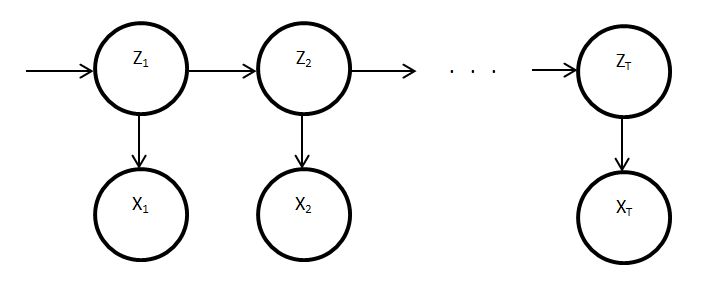
Thursday, 28 April 2011

Classification a single appliance's state using a hidden Markov model

The simplest scenario is one in which we wish to determine the state of a single two-state appliance, given its power demand. This can be represented as a hidden Markov model as follows:
where:
  • Zt - hidden (latent) variable at time t (appliance state)
  • Xt - observed variable at time t (power reading)
For a given set of observed variables, we can expand the possible chains of hidden variable states as a lattice diagram:
where:
  • k - appliance state
It can be seen from this diagram that the number unique chains of hidden variables through this lattice scales exponentially with the length of the chain. However, the max-sum algorithm (called the Vertibi algorithm in this case) can be used to find the probability of the most likely chain, with complexity that grows only linearly with the length of the chain. The values of the most likely chain can then be found by backtracking through the chain starting from the final time slice of the most likely chain.

The Viterbi algorithm involves calculating the joint probability of a chain of observed and hidden variables, given by:
where:
  • X - set of observed variables
  • Z - set of hidden variables
  • theta = {pi, A, phi} - model parameters
  • pi - probability density of z1
  • A - appliance transition probability matrix
  • phi - emission density (probability density of observed variable given a hidden variable)
  • N - number of time slices
The model parameters parameters can be learnt from the set of observed variables using the Expectation-Maximisation algorithm. However, we may want to introduce a prior belief over some parameters, or even fix some parameters. For example, we might know the state of the appliance at the start of the chain, and can therefore fix pi. We might also know the parameters governing the emission density, and if we assume the observations are normally distributed we might want to fix the mean and variance parameters of the Gaussian function.

Although this model can represent appliances with more than two states, it is unclear how tractable the EM algorithm will be for a factorial hidden Markov model. One solution would be to model the multiple Markov chains as a single Markov chain, whose number of states is equal to the number of combinations of appliance states. However, the complexity of such a model is then exponential in the number of appliances. It is worth noting that we can prune the number of possible transitions based on the assumption that only one appliance can change state between two consecutive time slices, which is a practical assumption assuming a small time interval between time slices. A solution to solving this might be to use sampling methods.

Friday, 15 April 2011

NIALM as a factorial hidden Markov model

After considering various heuristic approaches towards NIALM, it is clear that a more principled probabilistic approach is required. The approach would need to recognise that premise-level power readings are sequentially drawn from a continuous time series, and are not independent of each other. In fact, intuition tells us that in general appliances are far more likely to stay in their current state, and that state changes are comparatively rare. NIALM can also be considered as an online-learning problem, in which disaggregation must occur after each individual premise-level power value has been received. These two assumptions map directly on to the modelling of such a problem as a factorial hidden Markov model.

In a factorial hidden Markov model, there are multiple independent chains of hidden variables, which in this case are the current operating state of each appliance. At each time slice, there is also an observed variable conditional on the states of all of the corresponding hidden variables, which in the case is the premise-level power value. Below is a diagram of a factorial hidden Markov model.

where:

  • Z - hidden (latent) variable, subscript - time slice, superscript - variable number
  • X - observed variable, subscript, time slice
NIALM solutions are interested in evaluating the state of appliances, and given a look-up table of appliance state power values, can therefore evaluate the power of each appliance at each time slice. We are therefore interested in modelling the probability of an appliance being in a certain state, given the appliance's state in the previous time slice and the observed variable for that time slice:
This is an approach I will be investigating over the following weeks, after reading up on the relevant theory on sequential data and expectation-maximisation.

NIALM as a combinatorial optimisation problem - continued

As previously discussed, appliance loads can be disaggregated from premise-level power readings by the minimisation of a function f at each time slice:

where:

  • Pagg - premise-level aggregate power
  • N - number of appliances
  • I - vector of appliance binary indicators (1 if appliance is on, 0 otherwise)
  • P - vector of appliance power when appliance is on
Two commonly cited disadvantages of this approach is how its accuracy would decrease with the number of appliances and level of noise. However, no research has been published investigating the situations in which this approach performs sufficiently accurately. I have tested this approach using simulated data for 24 time slices, relating to one reading per hour over the course of a day. Below are tests evaluating the performance of this approach as the number of appliances is increased and as the noise in the data is increased.

Increasing numbers of appliances

Below shows a graph of this approach's true positive rate (TPR) and false positive rate (FPR) for increasing numbers of appliances, n. No noise was introduced over the simulated data set.


We can see that this approach performs very accurately from n = 1 to roughly n = 10. However, for n > 10 the TPR rapidly decays towards 0.5, while the FPR increases towards 0.25. This approach is clearly only useful for small n (roughly n < 20). However, it might be interesting to evaluate the performance of this method given only a small subset of appliances and the premise-level aggregate power. The appliances should be chosen such that they are the most power hungry appliances.

Increasing noise

To investigate how the accuracy of this approach is affected by noise, Gaussian noise was added to the premise-level power readings of the form:
where:
  • N - Gaussian distribution
  • x - Noisy premise-level aggregate
  • Pagg - actual premise-level aggregate
  • c - noise level
Below shows a graph of this approach's true positive rate (TPR) and false positive rate (FPR) for increasing noise in the aggregate power reading, c.


We can see that instantly after introducing some noise, the TPR rate drops to roughly 0.7 for Gaussian noise of standard deviation just 0.1% of the aggregate power level. It is clear that this approach is not robust to even small levels of noise in the premise-level aggregate power readings, as would be likely in a realistic setting.

Extensions

Two extensions are discussed below which could increase the accuracy of this approach.

First, the assumption that an appliance has only one state for which it can draw power can be relaxed. Instead, we allow appliances to operate in one of a number of K states, each of which has a unique power value. The appliance state indicator variable would therefore be a binary vector taking the form of a 1-of-K coding scheme, such that:
and
The optimal appliance combination would therefore be given by minimising the function f at each time slice:

Second, the assumption that appliance states at each time slice are independent of each other can be relaxed. This allows us to take into account information of known appliance lengths in the form of constraints, e.g. 10 minutes < fridge_cycle_duration < 20 minutes. However, this would significantly increase the complexity of the optimisation problem by including the additional time dimension.

Friday, 1 April 2011

NIALM as a combinatorial optimisation problem

NIALM can be formulated as a combinatorial optimisation problem as follows:

For each time instant, minimise the function f:
where:

  • Pagg - household aggregate power
  • N - number of appliances
  • I - vector of appliance binary indicators (1 if appliance is on, 0 otherwise)
  • P - vector of appliance power when appliance is on
This approach was first proposed by Hart, as explained in the 1992 seminal paper on NIALM. Hart asserts that this is an NP-complete "weighted set" problem, and mentions that the number of combinations of 'on' appliances scales exponentially with the number of appliances. However, despite its computational difficulty, the optimal solution can be found within seconds for a realistic number of appliances, e.g. 30.

I have recently been investigating the performance of this technique using simulated data. 24 hours worth of truth data was generated using 30 appliance profiles, each with realistic power demands and usage patterns. The true household aggregate was calculated by summing the power consumed by each device at that time instant. No noise was added on appliance nor household level.

I have been investigating how the performance of this technique decays as the number of appliances in the household increases. The optimisation function was applied at 1 hour intervals to 24 hours of data, and the accuracy was calculated as the average fraction of correct classifications.

Below is a graph showing the accuracy of this technique for the number of appliances in the house.


The technique is very accurate when there is less than 10 appliances in the household. Although the accuracy starts to drop rapidly, if seems to converge around 0.5 or 0.6. However, further tests of large numbers of appliances are necessary to prove this.

Obvious future work is to investigate how the performance of this approach decays with the introduction of appliance and aggregate level noise to the data.

Monday, 21 March 2011

My electricity consumption separated into lighting and appliances

I've recently been monitoring my electricity consumption using two AlertMe clamps round my household aggregate and lighting circuits. The graph below shows the power draw for Sunday 20.03.2011.


It is interesting to note how easy it is to recognise some specific appliances.
  • Fridge - 35-40 cycles throughout the day. The fridge's square power draw is clearly visible throughout the night, and at various points throughout the day. However, it is less obvious in the evening when many other appliances are operating.
  • Kettle - 10.00, 13.00, 17.30, 19.00. The kettle is distinguishable by its power draw of 2.5kW and its short duration for 2-3 minutes.
  • Washing machine - 13.00, 15.30. The washing machine has an alternating power draw between 600W and 0W for its 1 hour cycle duration. However, it also has a solid power draw of 2kW for about 20 minutes.
  • Oven - 18.30-19.30, 21.30-22.30. The oven's temperature is regulated by a thermostat so its power draw predictably alternates between 0W and 2kW. However, there is a period while it initially heats up to temperature when it is on continuously. For the first use the temperature was set to 170 degrees, while for the second use it was set to 110 degrees. This is reflected by the duration between 'on' cycles, similar to Alex's fridge's behaviour.

It is also interesting to analyse the lighting circuit's power draw. Since each light only has two states, 'on' and 'off', techniques such as steady-state analysis or combinatorial optimisation would work well here.

Friday, 11 March 2011

Bayesian modelling of appliance detections using smoothness metrics and cycle frequency

Previously, I discussed the use of Bayesian modelling for appliance signature matching. Following Bayes rule, the posterior is proportional to the product of the prior and the evidence:
where:
  • X = candidate appliance cycle corresponding to actual appliance cycle
  • t = time between known previous appliance cycle and candidate appliance cycle
The prior, P(X), will be calculated using a combination of smoothness metrics. The evidence, P(t|X), will be calculated using the known probability distribution of times between appliance cycles. These are explained respectively below.

Prior: P(X)

So far, I have proposed three metrics for assigning a confidence value to a possible appliance cycle. When defining them, I'll use the following notation:

  • P = Aggregate power
  • A = Appliance power
  • Q = P - A
  • t = time instant from 1 to T

1DERIV:
Difference between the sum over the first derivative of the aggregate power and the first derivative of the aggregate-appliance power:


2DERIV:
Difference between the sum over the second derivative of the aggregate power and the second derivative of the aggregate-appliance power:


ENERGYRATIO:
Ratio of the energy consumed by the appliance during its cycle and the energy consumed by all other appliance's during the cycle:
where:

  • a = time instant of cycle start
  • b = time instant of cycle end

Evidence: P(t|X)


We know the probability distribution of the time between appliance cycles. This is shown by the histogram below:
This can be modelled using a normal distribution of mean and standard deviation calculated from this data set. This model will be used to calculate the evidence probability.

Posterior: P(X|T)


I have calculated the posterior using two combinations of smoothness metrics to form the prior:

  1. threshold(1DERIV) * 2DERIV
  2. threshold(1DERIV) * ENERGYRATIO
In both cases, the 1DERIV metric has been used to calculate whether subtracting the appliance signature had smoothed the aggregate power array. A threshold was applied to these smoothness values to produce a list of candidates for which the subtraction increased the smoothness of the array. Next, the candidates were multiplied by a confidence metric. In the first case the 2DERIV metric was used, and in the second case the ENERGYRATIO metric was used.

Given a known appliance cycle and a number of candidates for the immediately following cycle, the posterior probability for each candidate cycle was calculated. The maximum likelihood candidate cycle was selected as a correct cycle and the process was repeated sequentially for the remaining cycles.

The two plots below show the estimated fridge cycles (blue) against actual fridge cycles (red).

1. threshold(1DERIV) * 2DERIV

2. threshold(1DERIV) * ENERGYRATIO


Both estimations worked well, correctly detecting 23 and 24 cycles respectively, out of 31 actual cycles. Each method actually only generated 30 positives, of which 7 and 6 were false positives respectively. There was a common interval in which neither approach generated a true or false positive, occurring at a time when the off duration was at a minimum. The use of a model with an off duration that varies over time might increase the performance of both approaches here.

In addition, it is interesting to note that there are some areas where approach 1 outperforms approach 2, and other areas where approach 2 outperforms approach 1. This is encouraging, as it could mean that the two approaches are complementary. I investigated using a third approach in which the confidence metric was the product of 2DERIV and ENERGYRATIO, although the result was less accurate than either individual approach.

Thursday, 10 March 2011

More smoothness metrics

Recently I've been looking at whether subtracting an appliance's known signature from the aggregate demand increases the smoothness of the curve. The success of such an approach is clearly dependant on what smoothness metric is used. I've already looked at the sum of the changes in power:
This is equivalent to taking the first derivative if the power values, because the denominator, dt, is always 1.

However, recently I've been troubled by the way this metric indicates an optimal match for the five graphs shown below. They are all possible combinations of the fridge's signature (red) with other appliances (blue). The vertical corresponds to power (W) while the horizontal corresponds to time (minutes).

However, we'd prefer the metric to return an optimal match for graphs A-D, and a sub-optimal match for graph E. This is because it is far less likely that another appliance of the same duration as the fridge will coincide with both the fridge's 'on' and 'off' transitions.

In an effort to quantify this, I realised that subtracting the fridge's signature reduces the number corners in graphs A-D, but not in E. Since a corner corresponds to a change in gradient, the second derivative of P might be a useful metric for smoothness:
The absolute value of the second derivative of P with respect to t will produce a positive value corresponding to each corner, and 0 otherwise. Therefore, the number non-zero values produced by this function is a measure of the noisiness of a curve. Taking the reciprocal provides us with the desired smoothness metric.