As explained in previous posts, we can model the conditional probabilities of appliance states and aggregate power readings using a Markov chain of latent variables:
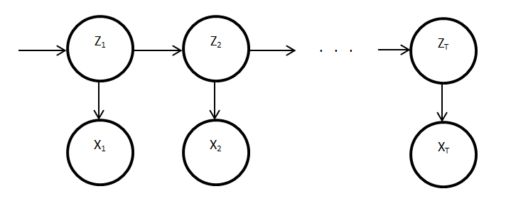
where:
- Zt - discrete latent variable at time t (appliance state)
- Xt - continuous observed variable at time t (power reading)
This model can be manually trained by specifying the model parameters:
- pi - probability density of z1 (probabilities of initial appliance states)
- A - appliance transition probability matrix
- phi - emission density (probability density of observed variable given a hidden variable)
The problem of non-intrusive appliance load monitoring can be formalised as:
Given a sequence of observed power readings, X, determine the optimal sequence of appliance states, Z, responsible for generating such a sequence.
The probability of a sequence of appliance states and power readings can be evaluated using:

As previously described, the optimal sequence of appliance states can be found using the Viterbi algorithm.
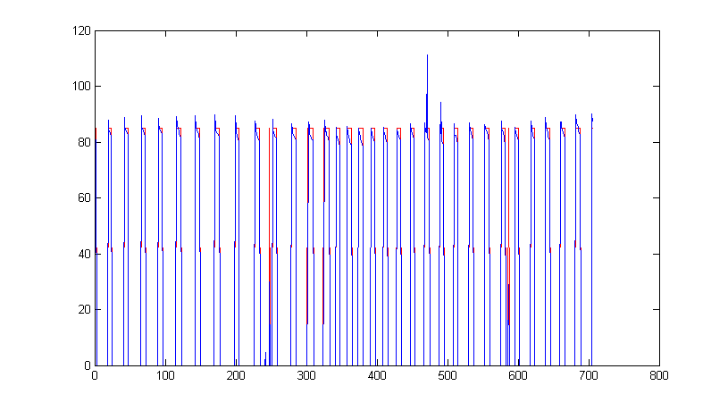
I have used the Bayes Net Toolbox for Matlab to model a single two-state appliance. The model is manually trained by specifying the model parameters pi, A and phi. It is then possible to sample realistic data of arbitrary length from the model. In addition, it possible to evaluate the probability of a sequence of appliance states and power readings. Therefore, the Viterbi algorithm can be used to find the optimal sequence of appliance states for an observed sequence of power readings. I have implemented the Viterbi algorithm and used it to calculate the optimal sequence of states for a fridge, given a sequence of the fridge's power readings. Below is a graph showing the fridge's power reading (blue) and the estimated appliance states (red), where 85 represents on and 0 represents off.
In this case of a single two-state appliance, this approach performs similarly to simply comparing the power samples, p, against a threshold, x, where p > x indicates the appliance is on, and off otherwise. However, using this probabilistic approach has advantages over such a heuristic approach. The threshold method would always estimate the appliance be on if the power reading is above a given value, and therefore treats the data as independent and identically distributed. Conversely, the probabilistic approach takes into account the appliance's previous state and the probability of it changing state, and therefore exploits the sequential nature of the data.
This method is easily extended to a single appliance with more than two states, an approach which I intend to explore in the near future. This method can also potentially be extended to many appliances with multiple states, an approach that I intend to explore in the more distant future.
